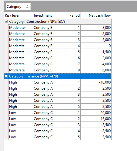
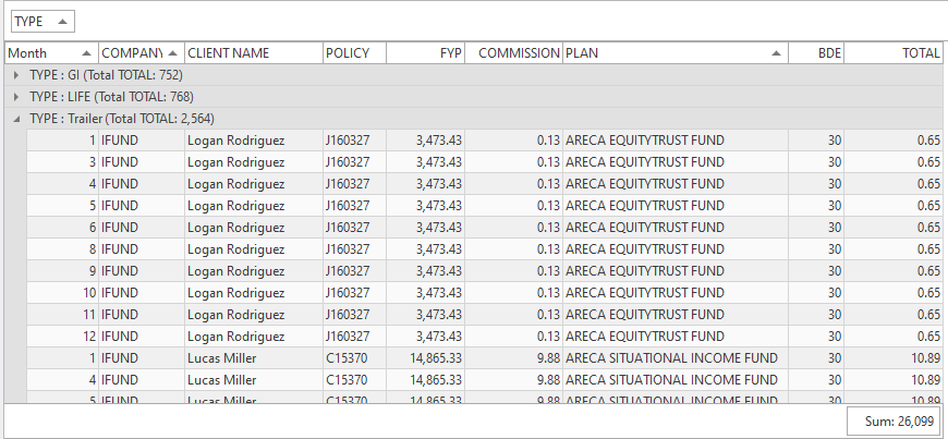
In this walk-through, we will be importing data from 13 Excel files containing financial transactions. The end-result will allow us to compute summary values for a single grouped column e.g.
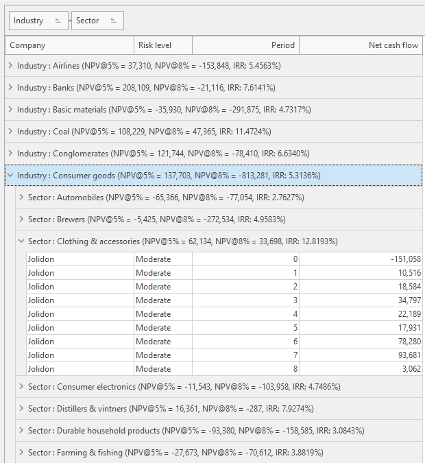
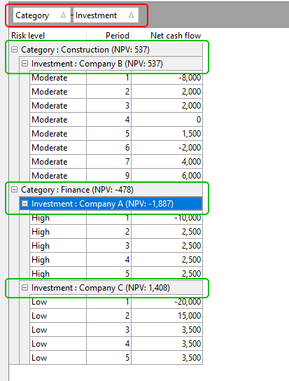
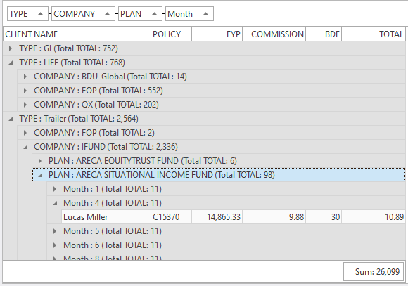
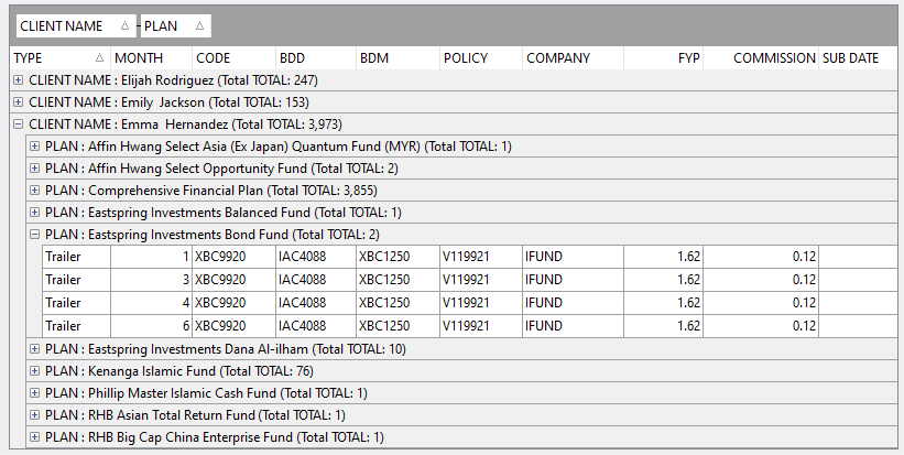
and for multiple levels of grouping e.g.
or
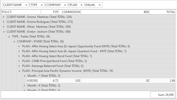
Prerequisites
Install Easy Excel Analysis using the installer located here.
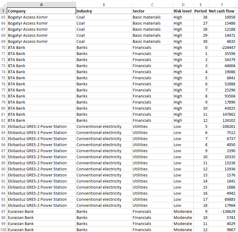
The source Excel files
Our source files consist of 13 Excel files, each containing data for one month, except for February which consists of 2 files.
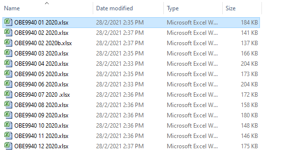
Note that the each file identifies the month the data belongs to in its naming convention e.g. OBE9940 01 2020.xlsx indicates that the data in this file is for January, and OBE9940 12 2020.xlsx is for December.
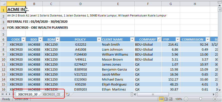
Each Excel file contains 2 worksheets. We will be importing data from the first worksheet.
Importing the data
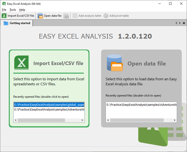
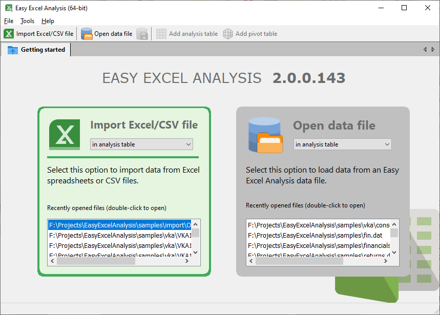
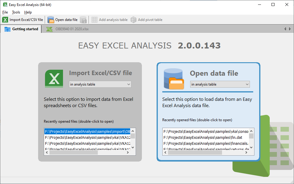
Open Easy Excel Analysis. Click on the Import Excel/CSV file box.
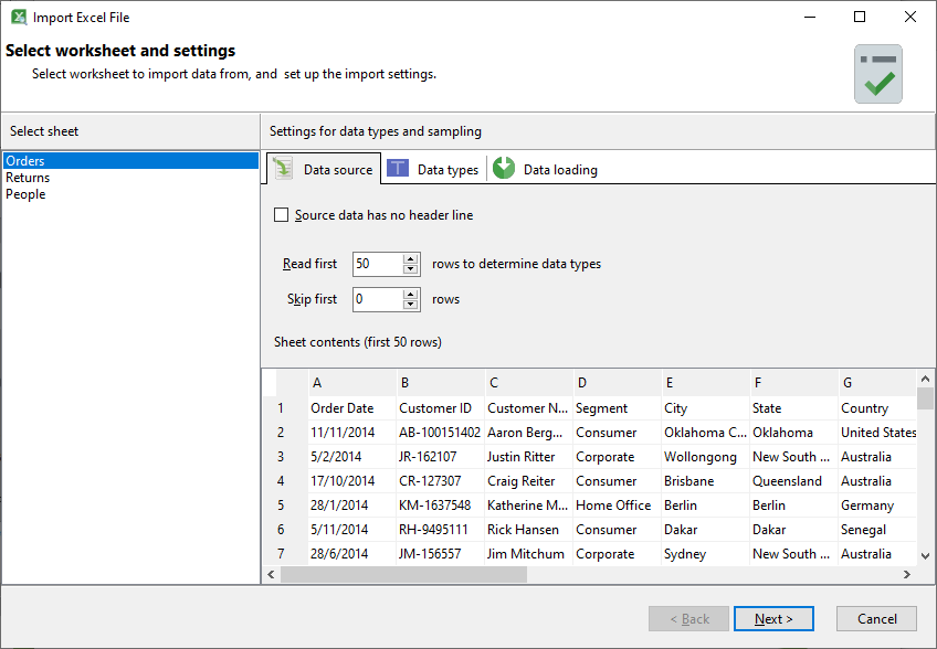
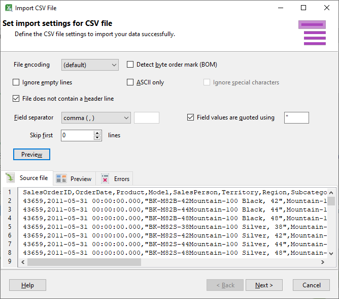
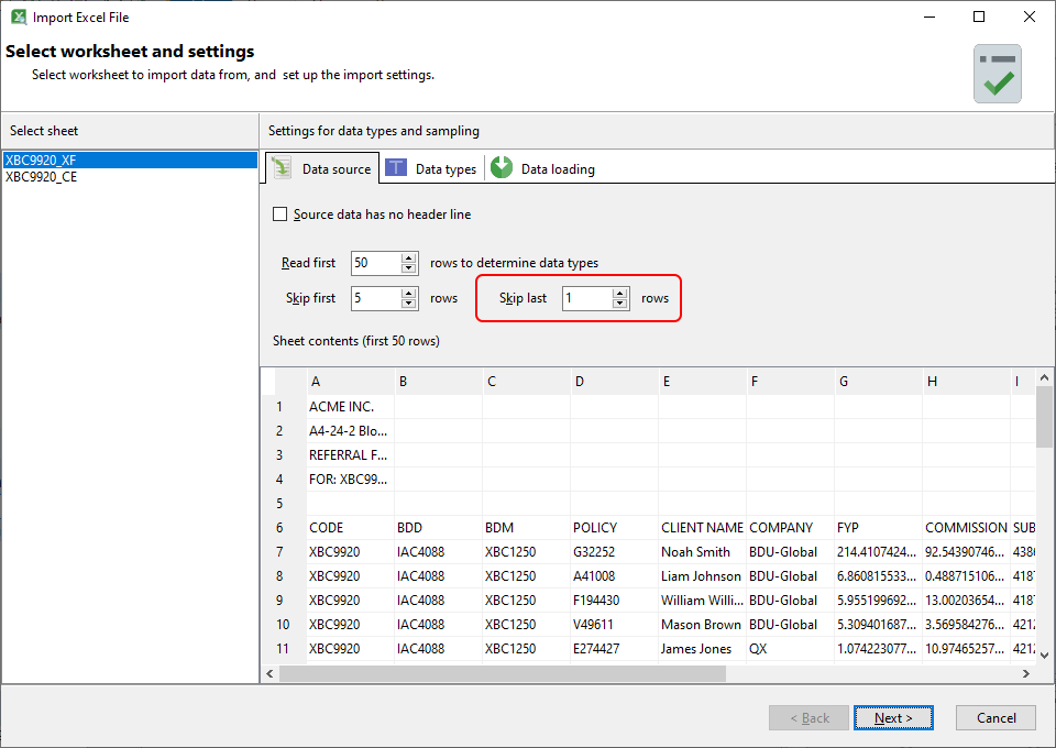
Select the first Excel file to import. This will be our primary source file. Easy Excel Analysis opens the file and displays the first 50 rows.
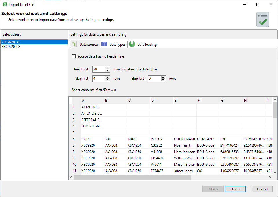
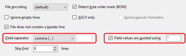
The list of available sheets are displayed on the left, and the first sheet is selected by default. Our source file contains some header details, and the actual data only starts from the 6th row.
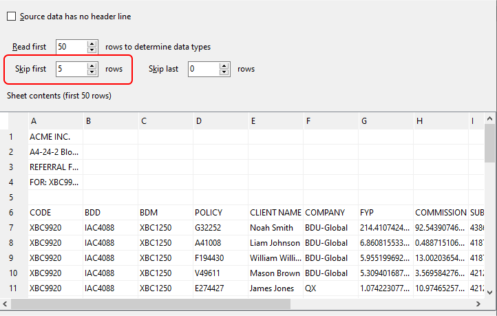
Thus, we need to set the Skip first value to 5.
Our source file also contains a total at the end of our data block.
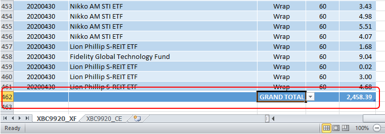
As we do not require this row, we need to set the Skip last value to 1 so that Easy Excel Analysis ignores this row.
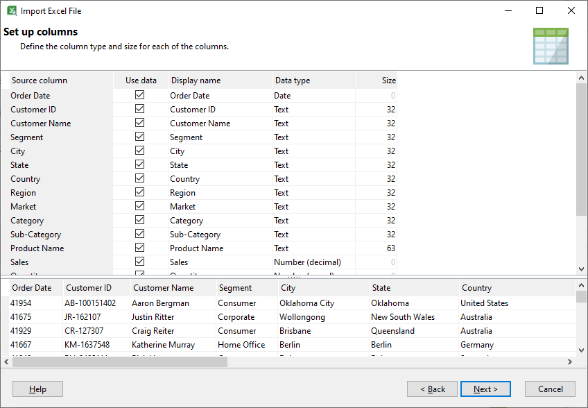
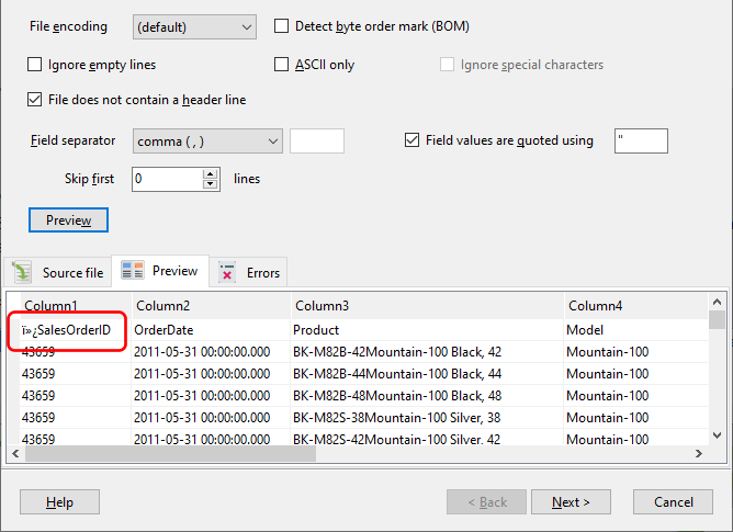
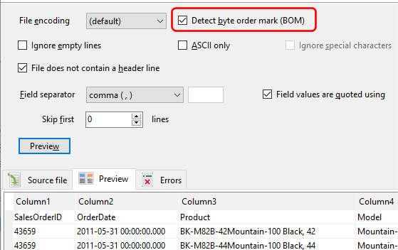
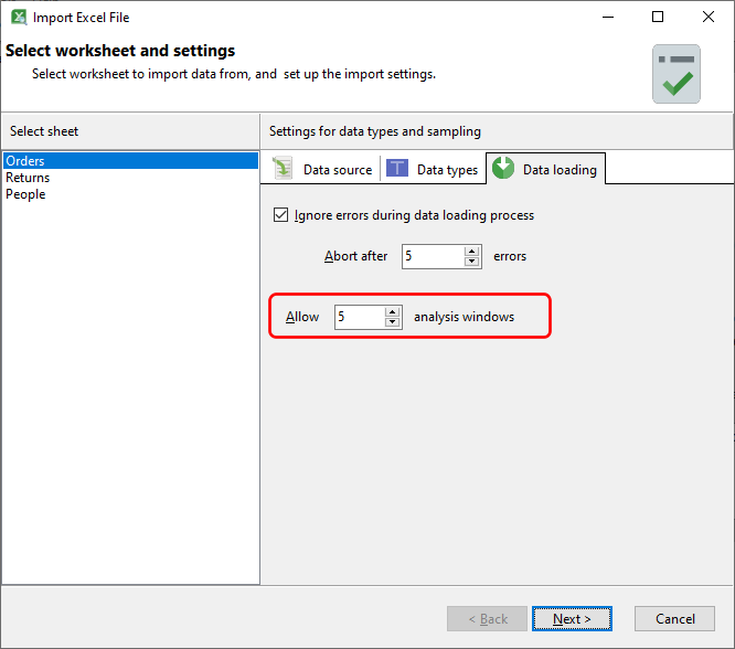
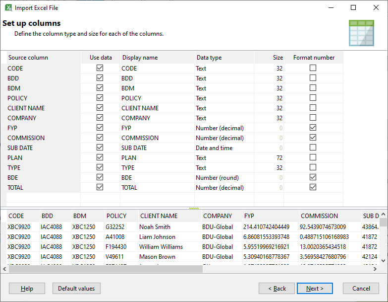
Click Next and ensure that the column types have been identified correctly.
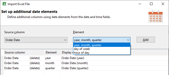
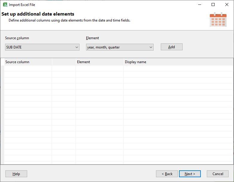
Click Next. Here, we can set up derived values from the date columns in our data set. We will skip this step.
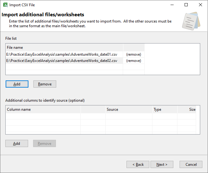
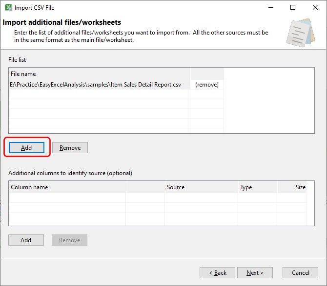
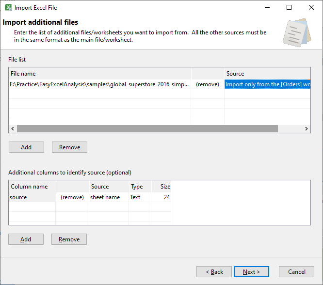
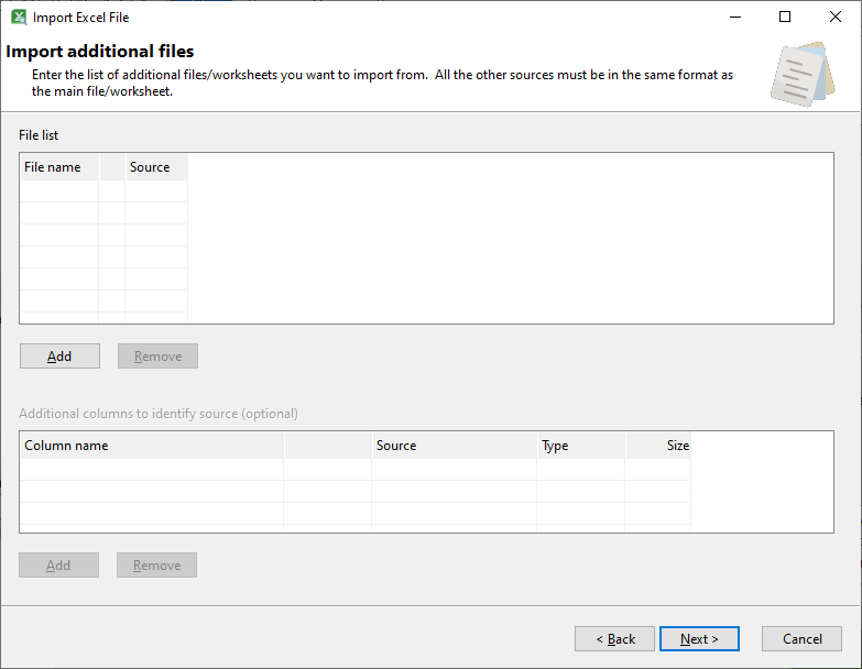
Click Next. Here, we can enter the other files we want to import. Click on the Add button.
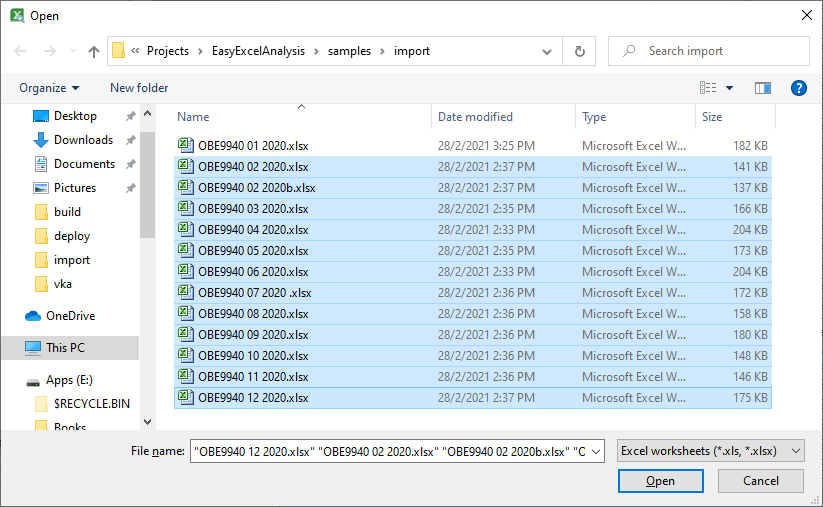
Select the files we want to import. You can use the CTRL and SHIFT keys when clicking on the file names to select multiple files. Click Open once you have selected the files.
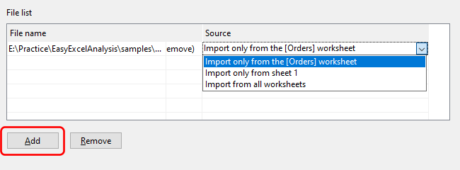
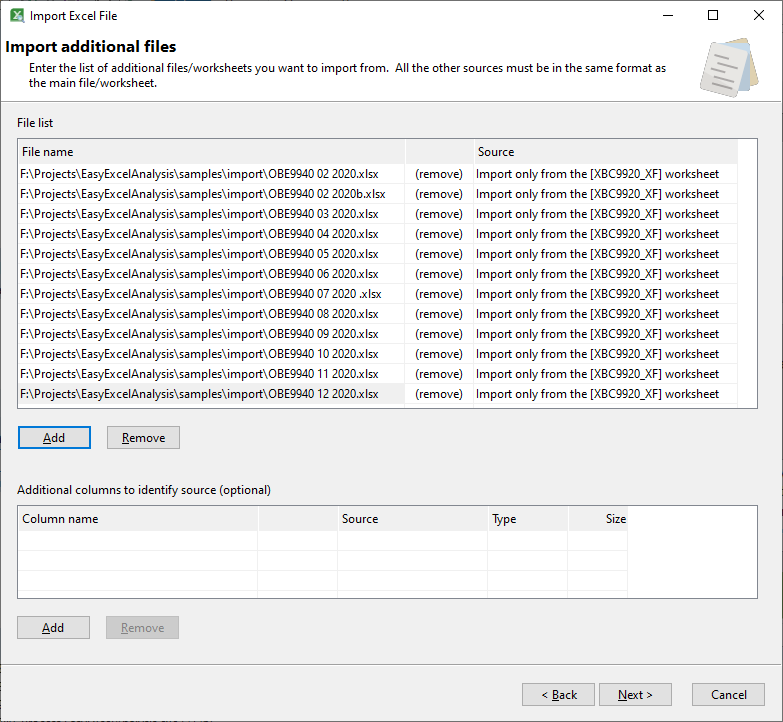
The selected files are listed, and the default option is to import the data from the sheet of the same name as our primary source file.
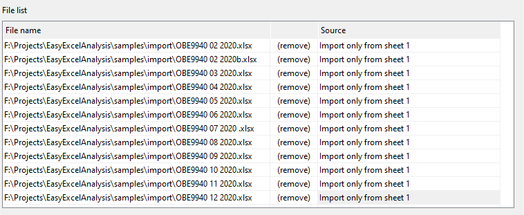
Unfortunately, our source files do not have a consistent naming convention with regards to the sheet names. Thus, we will need to change the import option to import only from sheet 1.
Our source files do not contain any values that identify the month each transaction. Thus, if we import the data now, we cannot identify which month the transaction belongs to. As this information is important to us, we need to add an additional column to our combined data.
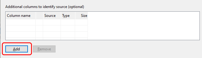
We can either open each worksheet and add a column containing the month value, or add a new column using Easy Excel Analysis. To do that, click on the Add button in the additional columns section.
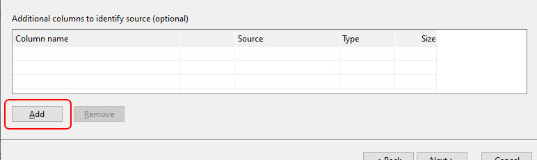
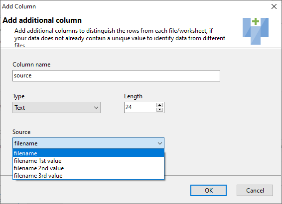
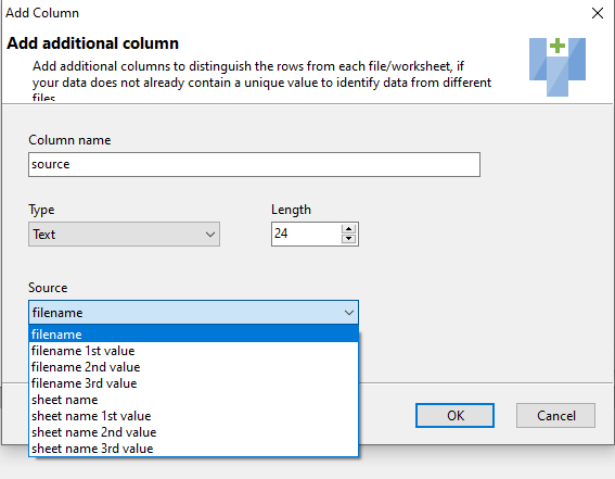
This brings up the Add additional column window.
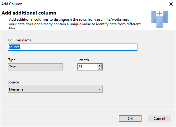
We will name this column MONTH. As we will be getting the value for this column from our file name (recall that our file names contain the numeric month value), we will specify a number type. The month value in our files names is the 2nd value, so we select the filename 2nd value as the source for this column.
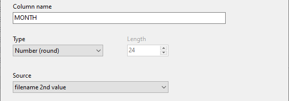
Easy Excel Analysis recognizes spaces, dashes, and underscores as separators for values, so any of these file names in our example would provide the correct month value.
- OBE9940 01 2020.xlsx
- OBE9940-01-2020.xlsx
- OBE9940_01_2020.xlsx
Click Next , and Easy Excel Analysis will then start importing from our primary source file and the additional files we listed.
Analyzing the data
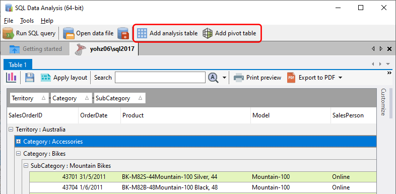
Once the data has been imported, you can start grouping and summarizing the values. Let’s start by creating a group summary value for the TOTAL column.
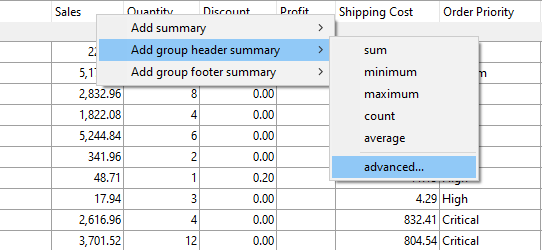
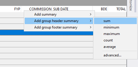
Right click on the TOTAL column header. Select the Add group header summary item, then the sum function.
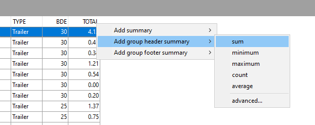
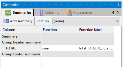
In the Summaries listing on the right panel, you should now see that a summary has been created for the TOTAL column, using the sum function.
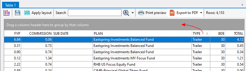
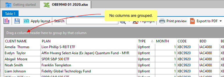
Now drag and drop the TYPE column header to the column grouping area.
The data rows are now grouped by TYPE, and the summary values calculated for each TYPE value.
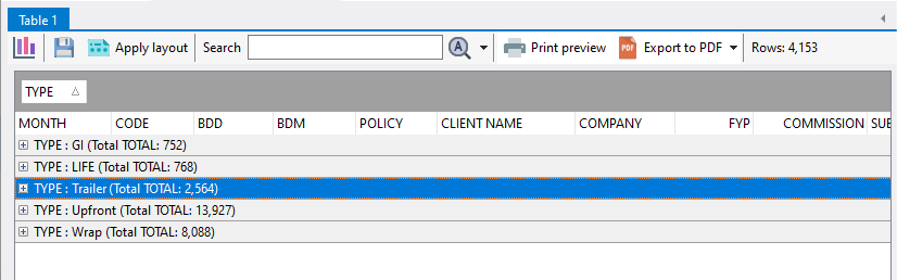
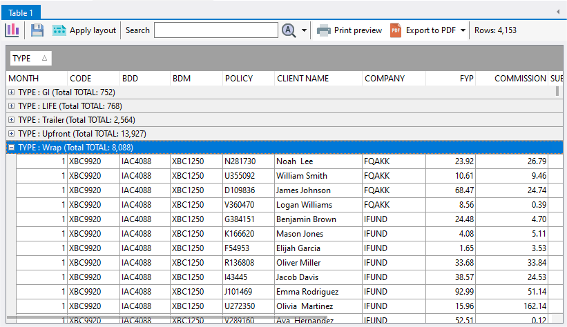
Expanding any of the TYPE value will display the details for that value.
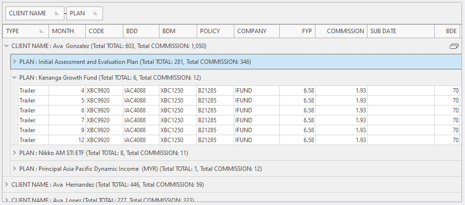
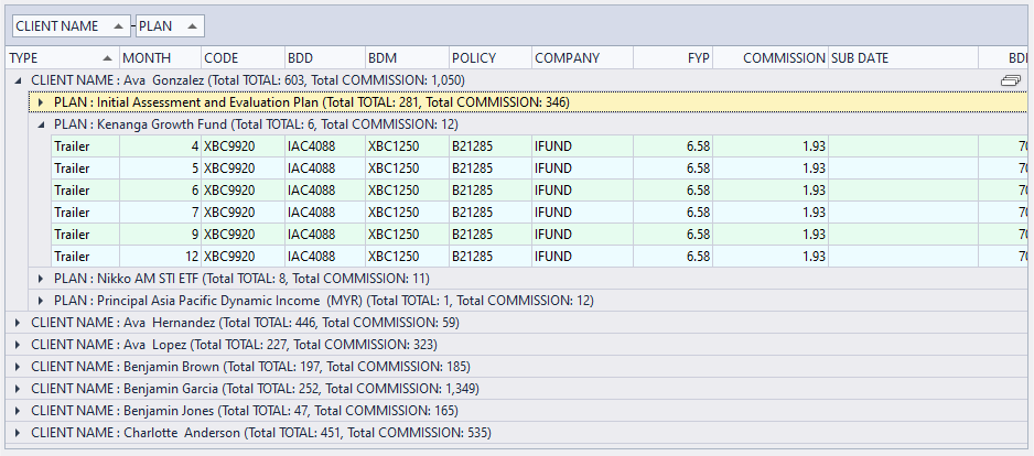
We can create as many grouping levels as we require simply by dragging and dropping the columns into the grouping area. Say we want to see how much we earn from each client, then by each plan. We just need to place the CLIENT NAME and PLAN columns into the grouping area.
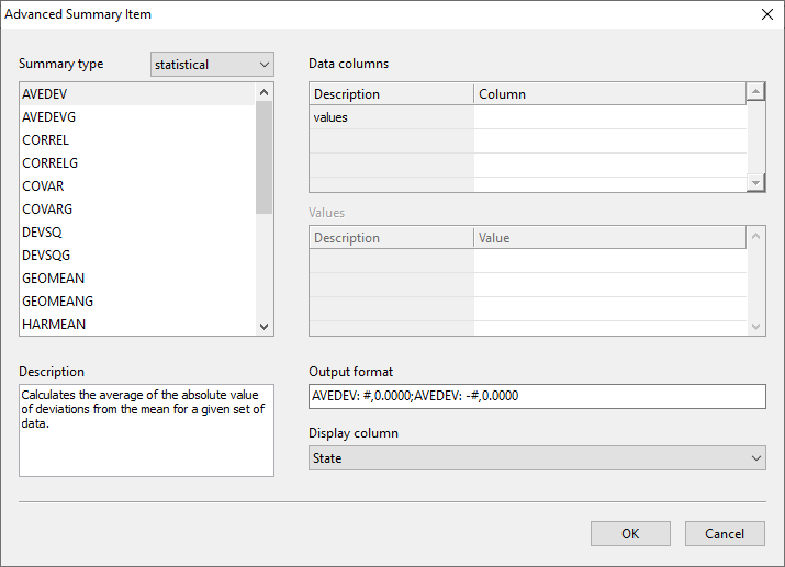
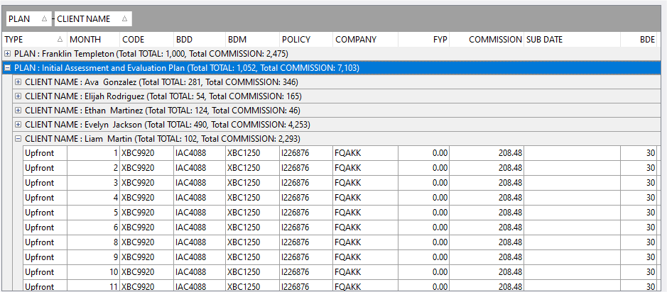
We can create additional summary values using the same steps for the TOTAL column. Say we want to display the total COMMISSION value at each grouping level. We right click on the COMMISSION column header, select the Add group header summary item, then the sum item.
The summary is then calculated and displayed immediately for each group.
Saving the grouping layout
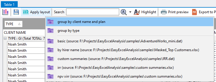
You can save each grouping layout by clicking on the Save current layout button.
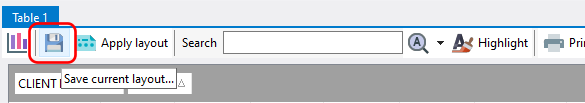
Enter a name for the layout. You can then later apply each saved layout by clicking on the Apply layout button and select the grouping layout you want to use.
Saving the data for future use
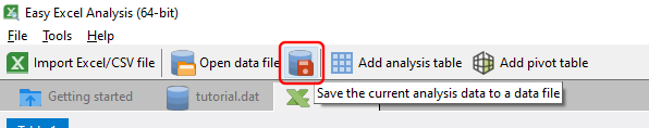
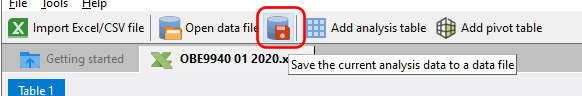
To save this consolidated data, click on the Save the current analysis data to a data file item, and enter a file name.
The next time you want to analyze this set of data, click on the Open data file box in Easy Excel Analysis and select the data file.
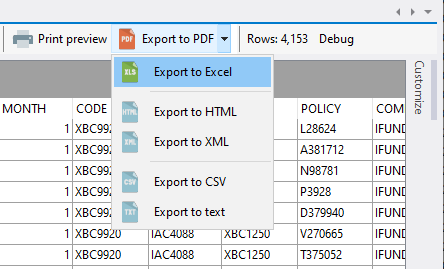
You can also save the consolidated data to an Excel worksheet. Click on the Export to Excel item in the Export options.
Enter the file name, and the layout or data option.
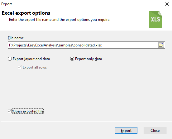
If you want to export only the rows without any grouping applied, ensure that your analysis table does not contain any grouping rows before you start the export.
Customizing the appearance
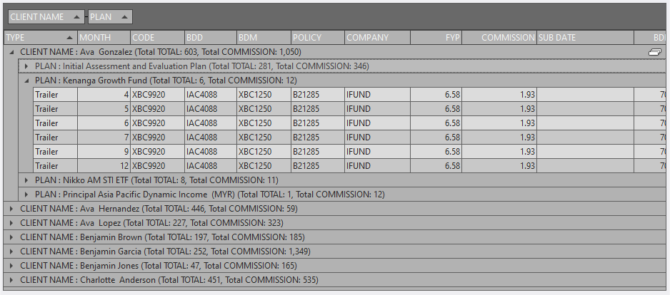
The Appearance tab on the Customize panel allows you to change the appearance of the displayed data.
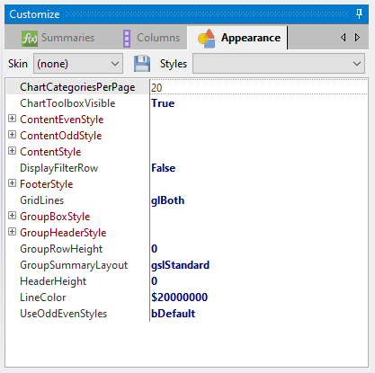
The Skin option allow you to quickly change the look of the data e.g.